Chapter 9 Crown Delineation

Supercells work to spatially group pixels with similar characteristics making it a great tool for crown delineation. The following workflow shows how to create and filter supercells into delineated crowns and requires:

1. A shapefile (.shp) with a grid of tree locations derived by georeferencing the census data to the imagery. This will be referred to as the “grid”. Detailed steps for creating the grid can be found in the chapter on georeferencing plot trees.

2. Co-registered CHM made from normalized maximum elevation (Z) values, MicaSense orthomosaic, and P1 orthomosaic, ideally from around the same date.

This workflow goes over:

• Loading in manually edited treetops (i.e. the “grid”) and creating circles proportional to a defined % of the tree’s height.

• Creating a supercell segmentation raster using the CHM and MicaSense and P1 orthomosaics

• Creating delineated crowns by filtering the supercells and merging remaining cells

• Cleaning the delineated crowns

We then highly suggest the crowns be reviewed and edited where necessary in a GIS to ensure the accuracy of future metrics calculated using the crowns.

9.1 Circles Proportional to Tree Height

The following code takes the grid and a registered CHM and creates a circle around each grid point that is proportional to a defined percent of its height. The percent will be dependent on the size and spacing of the plot trees.

In this example we decided to use 10% given the tight spacing and areas of crown closure. We recommend trying a range of percentages and choosing the one that gives proportional circles that contain as much of the visible portion of the crown as possible without also catching neighbouring branches.

Depending on the project, circles proportional to height may serve as adequate tree crowns however, if not, these circles will be used later in this workflow to filter the supercells to create defined crown boundaries.

Click to show the code

unique_id <- "TAG" # change this to the unique ID you have per tree that was used to create the grid
crown_dir <- paste0("path to save crown delineation producst to")# This was a path to a folder called Crowns for us

ttops <- st_read("path to your grid")# read in the treetops as an sp object
ttops<- ttops%>%
  st_centroid()

# Buffering circles around grid points to get heights for each tree:
buffer_radius <- 0.1  # buffer radius in meters
ttops_buffered <- st_buffer(ttops, dist = buffer_radius)# Create a buffer around each centroid with a radius of 10cm (0.1 meters)

#Check geometries, this should be  = 0
sum(!st_is_valid(ttops_buffered))

ttops_buffered <- ttops_buffered[!st_is_empty(ttops_buffered), ]

# Height Quantile from CHM
CHM_L1 <- "path to CHM" #path to CHM
CHM_max_L1 <- rast(CHM_L1) #read in CHM as a raster

extracted_values = ttops_buffered %>% #extract height percentiles
  exact_extract(x = CHM_max_L1,
                y = .,
                fun = "quantile",
                quantiles = c(0.975, 0.99),
                force_df = TRUE,
                append_cols = c(unique_id)) 

ttops_zq99 <- left_join(ttops_buffered, extracted_values, by = c(unique_id)) # Assign the pixel IDs to each polygon

# Saving out shp of buffered points
if(!dir.exists(paste0(crown_dir,"Buffer_radius_ttops_",buffer_radius))){
  dir.create(paste0(crown_dir,"Buffer_radius_ttops_",buffer_radius))
}
st_write(ttops_zq99, paste0(crown_dir,"Buffer_radius_ttops_",buffer_radius,"\\",site,"_ttops_",buffer_radius,"mBuffers_.shp"), append = FALSE)

# Proportional hulls based on 10% of the 99th percentile height value
percent <- 10
(buffer_dist <- ttops_zq99$q99 * (percent/100)/2)

buffer_dist[is.na(buffer_dist)] <- 0 

prop_hulls <- ttops_zq99%>%
  st_as_sf(crs = 26910)%>% #change to match your CRS
  st_buffer(dist = buffer_dist)%>% #value here is the radius
  mutate(buff = buffer_dist)

(prop_hulls$crownArea <- st_area(prop_hulls))

#Below we remove columns with mainly NAs as they will cause errors for the segmentation raster
prop_hulls_forSEG <- prop_hulls %>%
  dplyr::select(c(TAG, row, col, q99, q97, crownArea)) #select columns you would like to keep in your crown shapefile, if the columns contain NA values, remove them for the following segmentation steps and re-join the columns at the end


st_write(prop_hulls_forSEG, paste0(crown_dir,"Buffer_radius_ttops_",buffer_radius,"\\",site,"_proportional_Hulls_Diam",percent,"percent_zq99_forSEG_.shp"), append = FALSE) #Save shapefile of circles proportional to height for each tree

See Figure 9.1 below for an example of the above output.

Figure 9.1: A section of the P1 orthomosaic with red circles outlining the circles proprotional to 10% of the 99th height percentile for each plot tree and grid points representing the top of the plot trees shown in blue.

9.2 Supercell Raster

To generate supercells, we use a CHM, MicaSense orthomosaic, and a P1 orthomosaic. When possible we provide rasters from the same flight date. However, if that is not feasible we select a CHM, MicaSense, and P1 orthomosaic from flight acquisitions flown as closely together as possible. This ensures that the aerial perspectives of the tree crowns remain highly consistent across the three rasters, facilitating more accurate supercell segmentation.

Click to show the code

library(future) 
library(supercells)
library(RStoolbox)

crown_dir_folder <- "directory to save files to" #change to match yours
ms_path <- "path to MicaSense orthomosaic"
p1_path <- "path to P1"
prop_hulls <- prop_hulls_forSEG #created in the step above

Hulls = prop_hulls

bound = Hulls %>% #buffer hulls by 5m to get a bounding box to trim rasters with
  st_buffer(5)

# Reading in CHM, MS, and P1 rasters to make supercells
CHM_max_L1 = rast(CHM_L1) %>%
  crop(bound) %>%
  trim()
ms_ortho = rast(ms_path)[[c(1,6,9)]] %>% 
  resample(CHM_max_L1, method = "near") %>% 
  crop(bound)%>%
  trim
rgb = rast(p1_path)[[1:3]] %>% 
  resample(CHM_max_L1,method = "near") %>% 
  crop(bound) %>%
  trim

# Ensure crs match between rasters prior to stacking
crs(ms_ortho) <- crs(CHM_max_L1) 
crs(rgb)<- crs(CHM_max_L1) 
crs(CHM_max_L1) == crs(ms_ortho)

use = c( # Creating a SpatRaster, crs must match for this step
  CHM_max_L1,
  ms_ortho,
  rgb)

use[use > 60000] = NA # Filtering out noisy data

use2 = terra::scale(use)

writeRaster(use2, paste0(crown_dir_folder,"scaled_for_segments.tif"),
            overwrite = TRUE)

use3 = use2 %>% 
  ifel(CHM_max_L1 < .25 , 
       NA, .)

plan(multisession, workers = 6L)

seg = supercells(use3, step = 6, compactness = 5, iter = 50)

if(!dir.exists(paste0(crown_dir_folder,"HULLS"))){ #creating "HULLS" folder to save the below supercell .shp to
  dir.create(paste0(crown_dir_folder,"HULLS"))
}
st_write(obj = dplyr::select(seg, supercells, geometry), 
         dsn = paste0(crown_dir_folder,"HULLS\\",site,"_SEGS_step6_c5.shp"),
         driver = "ESRI Shapefile",
         append = FALSE)

Figure 9.2 shows the supercells (outlined in green) created by the above R code. These outlined areas indicate groups of pixels that the supercell algorithm has deemed similar between the CHM, MicaSense and P1 orthomosaics.

Figure 9.2: Supercells shown in green, with circles proportional to the 99th height percentile in red and grid points representing plot trees in blue

9.3 Filter & Merge Supercells

Above we found supercells across the site however now we need to filter for supercells that belong to tree crowns only. We do this by using the previously made circles proportional to height where supercells must be within the circle or intersect the perimeter in order to be kept, see Figure 9.3 for a visual. In our case, given that the trees are mature and tightly spaced we are not concerned with capturing lower branches in our crowns as they are not visible due to occlusion and would result in inaccurate spectral and structural metrics. Hence we created circles that were proportional to 10% of the 99th percentile per tree to help refine supercells to areas that were 1) visible from an aerial perspective and 2) had limited overlapping branches with neighbouring trees.

Click to show the code

library(smoothr) #for fill_holes
#Creating a folder to save files to, this was set up so that multiple tests could be run with different "percent" values 
if(!dir.exists(paste0(crown_dir_folder,"Prop_Diameter",percent,"%OfZq99"))){
  dir.create(paste0(crown_dir_folder,"Prop_Diameter",percent,"%OfZq99"))
}

chm_dat = c(CHM_max_L1)
names(chm_dat) = c("CHM_max_L1")

seg_extract = seg %>% 
  exact_extract(x = chm_dat,
                y = .,
                fun = "max",
                force_df = TRUE,
                append_cols = c("supercells"))

class(seg_extract)

seg1 = st_join(seg, prop_hulls_forSEG) %>% #joins supercells that are within or intersect circles to the circle dataset
  drop_na() %>% 
  left_join(seg_extract, by = c("supercells"))

saveRDS(seg1, paste0(crown_dir_folder,"Prop_Diameter",percent,"%OfZq99\\SEG_intersection.rds"))

st_write(obj = seg1, 
         dsn = paste0(crown_dir_folder,"Prop_Diameter",percent,"%OfZq99\\SEG_intersection.shp"),
         driver = "ESRI Shapefile",
         append = FALSE)

Figure 9.3: Supercells (outlined in green) filtered to only retain those that are within or intersect the cirlces propotional to height (red)

Below we show an example of further filtering the supercells. First we filter for supercells that overlap areas with a max height greater than a set threshold of 50% of the 99th height percentile using the CHM. This filtering step is mainly if you want to ensure you are only including data from above a certain height percentile in your crowns that was not already removed by the above filtering step using the proportional circles. In this example, no supercells were filtered out from this filter.

We then filter out supercells that are within two proportional circles (a.k.a. in two different crowns). The “supercells” column represents a unique ID for each supercell however in the st_join step above if a supercell intersected more than one proportional circle it will be recorded twice, once for each circle. Hence, we group the supercells by their unique ID (i.e. “supercells” here) and filter out supercells with more than 1 row. For example, in Figure 9.4 supercells highlighted in red are those where “count” = 2 ( so intersects two circles) and those highlighted in purple are cells where “count” = 1, we filter to only keep supercells where “count” = 1.

Click to show the code

seg2 = seg1 %>% 
  mutate(z50_L2 = q99 * .5) %>% #filtering out supercells where the CHM value in that super cell as less than 50% of the 99th percentile (~50th height percentile)
  mutate(TAG_archive = TAG,
    TAG = if_else(
    max > z50_L2, 
    TAG, 0)) %>% 
  group_by(supercells) %>% #group by supercells so you can filter for supercells within two circles
  mutate(count = n()) %>%  #number of rows in each supercell - this value should be 1, if it is two it means that the supercell intersected two circles 
  mutate(TAG = if_else(count > 1, 0, TAG))

st_write(obj = seg2, 
         dsn = paste0(crown_dir_folder,"Prop_Diameter",percent,"%OfZq99\\SEGS_initial.shp"),
         driver = "ESRI Shapefile",
         append = FALSE)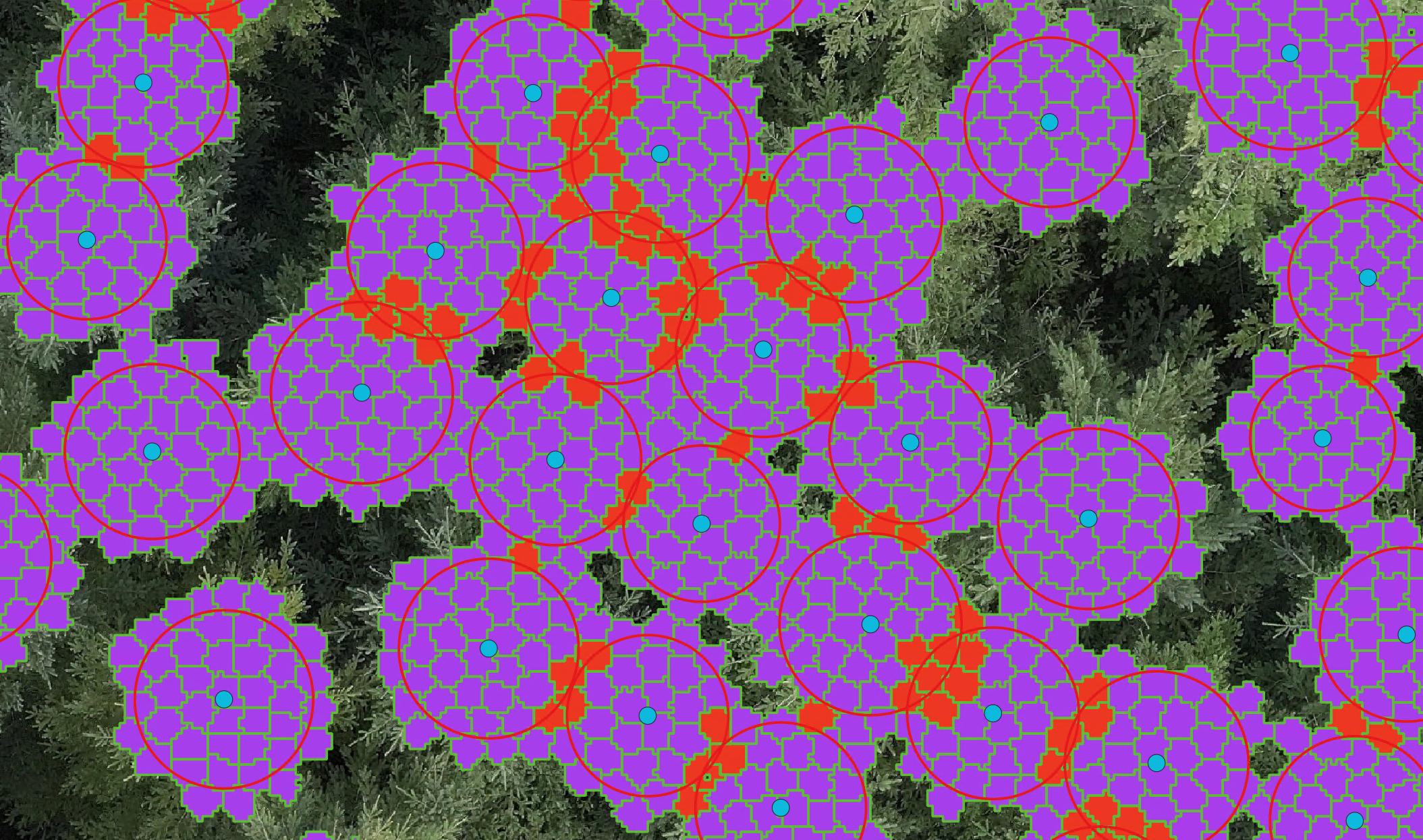

Figure 9.4: Supercells belonging to one proportional circle (purple) or two proportional circles (red). Those belonging to two proportional circles are highlighted in red and will be removed in the next step.

Next, we filter for supercells where TAG (the unique tree ID) is not zero, which implements the filtering from the above step. We then create center points, or centroids, for each supercell and filter for supercells with centroids within the proportional crowns. See Figure 9.5 for a visual of the supercell centroids that fall within the circles (yellow), boundaries of supercells with centroids that did not fall within the circle (green) and those that did fall within the circle (orange). This code filters to only keep the supercells outlined in orange.

Click to show the code

seg3 = seg2 %>% 
  filter(TAG != 0) %>% 
  st_centroid() %>% 
  st_join(y = prop_hulls_forSEG, join = st_within) %>% 
  drop_na() %>% 
  dplyr::select(supercells, geometry)

st_write(obj = seg3, 
         dsn = paste0(crown_dir_folder,"Prop_Diameter",percent,"%OfZq99\\SEGS_centroids.shp"),
         driver = "ESRI Shapefile",
         append = FALSE)

seg4 = seg2 %>% 
  st_join(seg3) %>% 
  drop_na() 

st_write(obj = seg4, 
         dsn = paste0(crown_dir_folder,"Prop_Diameter",percent,"%OfZq99\\SEGS_keep.shp"),
         driver = "ESRI Shapefile",
         append = FALSE)

Figure 9.5: Filtered supercells (green outline) that do not have a centroid that falls within it’s respective proportional circle. Supercells highlighted in orange do have a centorid that falls within it’s respective proportional circle, these are the supercells that will be retained and merged to form crowns in the following step.

Next we merge the supercells by TAG to create individual tree crowns, as seen in Figure 9.6 where the yellow outlines are the outwards boundaries of the merged supercells that form the tree crown.

Click to show the code

seg5 = seg4 %>% 
  group_by(TAG) %>% 
  summarise()
st_write(obj = seg5, 
         dsn = paste0(crown_dir_folder,"Prop_Diameter",percent,"%OfZq99\\SEGS_merge.shp"),
         driver = "ESRI Shapefile",
         append = FALSE)

Figure 9.6: Retained supercells (orange) merged to form crown boundaries (yellow).

The following two steps help clean the crowns. First, define a threshold value that represents the maximum area of a hole that you would like to fill within the crowns, here we chose 2000cm\(^2\). Figure 9.7 shows the crowns in yellow and the smoothed version of the crowns that have had holes filled in red. As you can see, the crowns are the same. This is because this section of crowns did not contain any holes that required filling.

Click to show the code

seg5_smooth <- seg5 %>% 
  fill_holes(threshold = units::set_units(2000, "cm^2"))

st_write(obj = seg5_smooth, 
         dsn = paste0(crown_dir_folder,"Prop_Diameter",percent,"%OfZq99\\SEGS_merge_smooth.shp"),
         driver = "ESRI Shapefile",
         append = FALSE)

Figure 9.7: Yellow crown boundaries are overlaid on top of crowns that have been edited to remove holes smaller than 2000 cm² (red). In this portion of the plot, no holes were present within the crowns, resulting in no visible differences between the original crowns (yellow) and those that have been refined through hole filling (red).

Next, we cast the crowns as polygons to remove instances of multipolygons associated with the same tree ID. Figure 9.8 displays the new polygons, outlined with blue dotted lines. Here we can see an instance of a smaller polygon shown in yellow and red that was originally grouped with the larger crown polygon within the circle, however has been filtered out in this step.

Click to show the code

seg5_smooth_NM <- st_cast(seg5_smooth, "POLYGON")
unique(st_geometry_type(seg5_smooth_NM)) # CHECK: should only have "Polygon" no more multipolygons
st_write(obj = seg5_smooth_NM, #saving out the crowns for manual editing
         dsn = paste0(crown_dir_folder,"Prop_Diameter",percent,"%OfZq99\\HULLS\\SEGS_merge_smooth_NoMultipolygon.shp"),
         driver = "ESRI Shapefile",
         append = FALSE)

Figure 9.8: Blue dotted lines represent crowns that have been converted to polygon class, overlaid on the original crowns in yellow and those with holes removed in red. In the upper center of the figure, a polygon (highlighted in red and yellow) that was initially part of a multipolygon within its proportional circle has been removed during the conversion to polygon in this step.

Lastly, we join the attributes from the original grid that contained information on each tree to the crowns shapefile.

Click to show the code

att <- ttops %>%
  as.data.frame()%>%
  dplyr::select(-c(geometry))

(seg5_smooth_NM_attributes <- left_join(seg5_smooth_NM,att, by = unique_id )) ## adding in attributes back

st_write(obj = seg5_smooth_NM_attributes, 
         dsn = paste0(crown_dir_folder,"Prop_Diameter",percent,"%OfZq99\\HULLS\\SEGS_merge_smooth_NoMultipolygon_Attributes.shp"),
         driver = "ESRI Shapefile",
         append = FALSE)

9.4 Manually Edit Crowns

Figure 9.9 is the final shapefile of delineated crowns from the above process. We then highly suggest the crowns be examined in a GIS and edited to remove sections where neighbouring branches intersect the crown to ensure each crown contains only data from the correct tree or to add in missed branches that are above your height cutoff. We recommend also adding a “crown confidence” column, or similar descriptive column, that can be populated throughout this process to mark partially obscured trees or any other instances that would lead to poor data quality down the line. This allows for these potential “problem” trees to be easily highlighted in future analysis. This was the most manually time-consuming process in the whole project.

Figure 9.9: Final crowns created using supercells and filtered with circles proportional to the height of each individual tree.