Chapter 13 MicaSense Irradiance Correction
13.1 Background
The MicaSense system measures radiance at the camera, which needs to be transformed into surface reflectance. The basic relationship is given by:
\[ R = \frac{L}{I_{\text{hor}}} \]
where \(L\) is the at-camera radiance and \(I_{\text{hor}}\) is the horizontal irradiance.
13.1.1 Deriving Horizontal Irradiance
Below we go through the derivation to compute \(I_{\text{hor}}\).
The MicaSense system includes both the cameras and a downwelling light sensor (DLS). Since the DLS is tilted at the angle of the drone during flight and the sun is rarely directly overheard the sensor, the DLS measures non-horizontal irradiance, referred to as spectral irradiance (\(I_{\text{spec}}\)). Spectral irradiance is a function of direct irradiance (\(I_{\text{direct}}\)), scattered irradiance (\(I_{\text{scattered}}\)), and the angle between the sun and the sensor ( \(\theta_{\text{sun-sensor}}\)):
\[ I_{\text{spec}} = I_{\text{direct}} \cdot \cos(\theta_{\text{sun-sensor}}) + I_{\text{scattered}} \]
If we take \(r\) to be the ratio of scattered to direct irradiance, \(r = \frac{I_{\text{scattered}}}{I_{\text{direct}}}\), we can substitute \(I_{\text{scattered}} = r \cdot I_{\text{direct}}\) into the equation:
\[ I_{\text{spec}} = I_{\text{direct}} \cdot \cos(\theta_{\text{sun-sensor}}) + r \cdot I_{\text{direct}} \]
Next, by factoring out \(I_{\text{direct}}\) from the equation:
\[ I_{\text{spec}} = I_{\text{direct}} \cdot \left( \cos(\theta_{\text{sun-sensor}}) + r \right) \]
We can solve for \(I_{\text{direct}}\) by dividing both sides of the equation by \(\cos(\theta_{\text{sun-sensor}}) + r\):
\[ I_{\text{direct}} = \frac{I_{\text{spec}}}{\cos(\theta_{\text{sun-sensor}}) + r} \]
If we assume that \(I_{\text{hor}}\) can be expressed in terms of \(I_{\text{direct}}\) with a similar function as seen above for \(I_{\text{spec}}\) however using the zenith angle, we can express this as:
\[ I_{\text{hor}} = I_{\text{direct}} \cdot \left( \cos(\theta_{\text{zenith}}) + r \right) \]
Substituting the equation for \(I_{\text{direct}}\) into the equation for \(I_{\text{hor}}\) gives:
\[ I_{\text{hor}} = \frac{I_{\text{spec}}}{\cos(\theta_{\text{sun-sensor}}) + r} \cdot \left( \cos(\theta_{\text{zenith}}) + r \right) \]
13.1.2 Calculating Reflectance
Finally, substituting \(I_{\text{hor}}\) into the equation for reflectance, we obtain:
\[ R = L \cdot \frac{\cos(\theta_{\text{sun-sensor}}) + r}{I_{\text{spec}} \cdot \left( \cos(\theta_{\text{zenith}}) + r \right)} \]
Thus we see that reflectance is highly dependent on the ratio of scattered to direct irradiance as well as the sun-sensor angle. This is important for understanding the issue we have found when working with the DLS2 and the MicaSense MX Dual camera system.
13.2 The Problem
The issue we have noticed is that the sun-sensor angle can be absurdly high or low, especially in strong illumination conditions. This leads to equally absurd, sometimes impossible, values for direct and scattered irradiance, that can be multiples higher than the direct solar irradiance.
To begin, let us first look at some main differences between the legacy DLS1 and the current DLS2 system.
The DLS1:
calculates the sun zenith angle using the GPS location of the drone and the time of acquisition
calculates the sun-sensor angle from the yaw/pitch/roll of the drone
The DLS2:
- directly measures the sun sensor angle and the direct and diffuse irradiance components using a proprietary method that takes in information from the light sensors on the surface of the DSL2
13.3 Is Correction Needed?
Deciding whether data needs to be corrected can be challenging. We have found that looking at these three questions can be helpful:
1) Do the sun sensor angles make sense?
2) Does the relationship between direct and horizontal irradiance make sense?
3) Does the scattered: direct ratio look right for the lighting conditions of that day?
Below we have plotted the sun sensor angle (top left), the position of each photo (bottom left) and the irradiance values (right) from the exif data of MicaSense imagery captured on June 25th, 2024 on Vancouver Island in British Columbia, Canada (Figure 13.1). We used yaw values to identify flight lines (blue and green) and roll to filter for images taken when the drone is turning (red). The black horizontal line is the calculated solar zenith angle at the time of the flight. This value was calculated using the latitude and longitude of the imagery and the time of day and was around 30°.
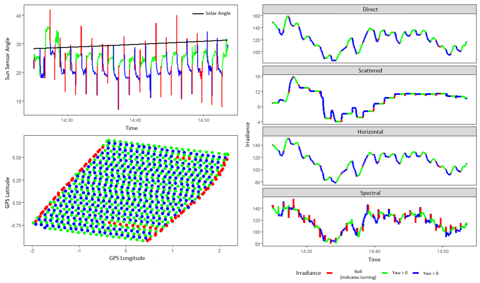
Figure 13.1: The sun sensor angle (top left), position of each photo (bottom left) and direct, scattered, horizontal, and spectral irradiance values (right) taken from the exif data of MicaSense images captured on June 25th, 2024 on Vancouver Island, BC, Canada. Flight line direction (blue and green) was identified using yaw values and images taken while the drone was turning were identified using roll (red).
13.3.1 Do the sun sensor angles make sense?
Solar zenith angle is the angle between the normal (vertical from the Earths surface) at the location of interest and the position of the sun. Given the tilt of the Earth, the solar zenith reaches its maximum (i.e. greatest angle between the sun and the normal to the Earths surface) in the winter, as the northern hemisphere is tilted away from the sun, and its minimum in the summer when the northern hemisphere is tilted towards the sun.
The solar zenith also changes throughout the day, with its minimum occurring at solar noon, a.k.a. when the sun is at its highest. This is why it is suggested to fly within ± 2 hours of solar noon to avoid shadows in your imagery.
Below we have graphed solar zenith angles over the winter solstice (December 24, 2024), summer solstice (June 21, 2024) and the date of the flight acquisition (June 25th, 2024) to demonstrate the daily and seasonal change in values (Figure 13.2).
The gray vertical bar highlights the flight time, which was just within the ± 2 hours of solar noon bounds and shows the solar zenith at around 30°, as we saw in Figure 13.1.

Figure 13.2: Solar zenith values plotted over the winter solstice (December 24, 2024), summer solstice (June 21, 2024) and the date of the flight acquisition (June 25th, 2024). Vertical lines indicate solar noon for the winter solstice (blue), summer solstice (red), and the duration of the drone flight (grey).
Now that we’ve refreshed our understanding of the solar zenith, let’s dive into the sun sensor angle. The sun sensor angle is, as it sounds, the angle between the normal (perpendicular) of the sensor and the direction of the sun (Figure 13.3). Given that drone flights occur relatively close to the ground compared to the distance from the Earth to the sun, this difference is often negligible. Therefore, the solar zenith angle can serve as a rough estimate of the sun sensor angle for a sensor that is parallel to the Earth’s surface - making it a helpful check to see if the sun sensor angle recorded by the DLS2 is within a reasonable range.

Figure 13.3: Visual representation of the solar zenith angle (left) and the sun sensor angle (right).
However, drones often fly at an angle, which can cause a cyclical pattern in sun sensor angles depending on flight direction. For example, let’s take a look at Figure 13.4. When the drone is flying in the general direction of the sun (left), the forward tilt of the drone mid-flight results in a smaller sun sensor angle compared to when the drone is flying away from the general direction of the sun, where the tilt of the drone away from the sun increases the sun sensor angle (right).

Figure 13.4: Schematic illustrating the impact of drone tilt during flight on the sun sensor angle.
This pattern of sun sensor angle dependence on drone orientation relative to the sun can be seen for the June 25th flight. Figure 13.5 shows the uncorrected sun sensor angles, derived from the DLS2 sensor located on the top of the drone, colored by flight line direction. Here red indicates turning and blue and green are opposite flight directions.

Figure 13.5: Sun sensor angles aquired from the DLS2 sensor colored by flight line direction.
Now that we understand the reason behind the cyclical pattern of the sun sensor angles, we can use the solar zenith value, plotted as the horizontal black line in Figure 13.5, to make an informed decision on whether the values need correcting.
To help this decision we recommend plotting the DLS2 sun sensor values and the sun sensor values calculated with the DLS1 method which will be referred to as the “corrected” values, see the section on sun sensor angle correction for the correction method.

Figure 13.6: Sun sensor angles over the flight duration from the DLS2 (purple) and corrected to mimic the DLS1 method (orange). Horizontal lines indicate the moving averages for the DLS2 (purple) and DLS1 (orange), where the balack line is the solar zenith calculated from GPS longitude, latitude, and time.
In Figure 13.6 the dashed horizontal lines are the moving averages of the sun sensor angles for the DLS1 and DLS2. Here the moving average of the sun sensor angles from the DLS2 is at times almost 10°lower than the solar zenith, whereas the moving average of the DLS1 (corrected method) is more or less consistently ~2-3° lower than the solar zenith.
Given this data, we would conclude that the DLS1 method provides more accurate sun sensor angles compared to the DLS2. We will now continue to look at irradiance to confirm if correction is needed.
13.3.2 Does the relationship between direct and horizontal irradiance make sense?
First, let’s define direct and horizontal irradiance with respect to the DLS:
Direct Irradiance: The direct component of the sunlight reaching the sensor’s surface that is not being scattered. On a clear sunny day, this component is high.
Scattered Irradiance: The sunlight that is scattered by particles in the atmosphere. This component is generally weaker on sunny days and higher on overcast days.
Horizontal Irradiance: The total irradiance on a horizontal surface, including both direct sunlight (projected onto the horizontal plane) and diffuse light. Hence, if the sun is directly above the sensor and it is a clear sunny day, the direct irradiance component will likely be quite close to the horizontal irradiance, however still lower given that horizontal irradiance includes diffuse light as well.
Below we have plotted the direct and horizontal irradiance from the DLS2 and values calculated with the DLS1 method (Figure 13.7 ). We can see that the direct irradiance from the DLS2 is greater than the horizontal irradiance, which is physically impossible. In contrast, the direct irradiance from the DLS1 method is approximately 50 W/m² less than the horizontal irradiance.
Explanations for the lower direct irradiance from the DLS1 compared to the horizontal irradiance include:
The ~30° sun sensor angle, which reduces the effective direct component captured by the sensor.
The portion of scattered irradiance in the horizontal irradiance signal that is not included in the direct irradiance value.

Figure 13.7: Direct and horizontal irradiance values throughout the flight from the DLS2 (purple) and corrected DLS1 method (orange).
From Figure 13.7, we would recommend correcting the data using the DLS1 method outlined below.
13.3.3 Does the scattered: direct ratio make sense for the lighting conditions of that day?
For a clear sunny day around solar noon, direct radiation generally accounts for ~85% of the total insolation with scattered radiation accounting for the remaining ~15%. For a completely overcast day, scattered radiation contributes to 100% of solar radiation.
Hence, for a clear sunny day in the summer a ratio of 1:6 scattered to direct irradiance is often used as an estimate. This means that direct irradiance is around 6 times stronger than the scattered irradiance.
Irradiance data plotted in Figure 13.8 from June 25th was captured on a sunny day with occasional light clouds.

Figure 13.8: Direct and scattered irradiance values throughout the duration of the flight from the DLS2 (purple) and corrected DLS1 method (orange).
The scattered: direct ratio for the data plotted in Figure 13.8 is ~0.09 for the DLS2 and ~0.46 for the DLS1.
DLS2: The ratio of 0.09 scattered: direct components from the DSL2 states that the direct irradiance during the flight was ~11 times greater than the scattered irradiance, or in other words that 91% of the total radiation reaching the earth was direct radiation and 9% was scattered radiation.
DLS1: The ratio of 0.46 scattered: direct components from the DLS1 states that the direct component was 2.17 times greater than the scattered component, hence 46% of the solar radiation was from the scattered component and the remaining 54% from the direct component.
Given that the flight on June 25th was flown just at the end of the 2 hour solar noon window under a sunny sky with the occasional cloud, we would assume that the scattered component would be greater than the minimum ~15% for fully clear skies at solar noon. Hence a value of 46% scattered radiation could be the result of extra scattering by the occasional clouds and a slight increase in scattering from a greater solar zenith angle. Overall, the value of 0.46 is more logical than the value of 0.09, since 0.09 implies less scattered radiation than the generally accepted minimum scattered component percentage on a clear sunny day.
Overall, we recommend correcting this flight using the DLS1 method. The DLS1 corrections are done on individual photos, if the orthomosaic has already been built, you can re-upload the imagery, re-calibrate, and re-build the orthomosaic in metashape without needing to reprocess the dense cloud.
13.4 Correcting Irradiance Values for MicaSense Cameras
This chapter explains the process of correcting irradiance values for MicaSense cameras using R. The correction involves several steps, including filtering and mutating data, calculating solar angles, and estimating scattered to direct light ratios. Each step is crucial for ensuring accurate irradiance readings, which are essential for downstream analyses. The code was taken largely from MicaSense’s GitHub and converted into R to use in our workflow.
To fix the sun-sensor angle and irradiance values we have taken the methodology used by the DLS1. The process involves:
Using the GPS location and time of acquisition to determine the solar zenith angle, and the yaw/pitch/roll of the drone to determine the sun sensor angle
Generating a rolling regression of the relationship: \(I_{\text{spec}} = I_{\text{direct}} \cdot \cos(\theta_{\text{sun-sensor}}) + I_{\text{scattered}}\) to determine the direct/ scattered irradiance ratio, \(r\), and only keeping realistic models with good fits
Computing the horizontal irradiance using \(I_{\text{hor}} = I_{\text{direct}} \cdot (cos(\theta_{\text{zenith}}) + r)\)
Editing the exif data of the images so that the imagery can be processed by Metashape with the corrected irradiance values
13.4.1 Reading Exif Data
First, we read in the exif data of the imagery we want to correct using the exifr package.
Click to show the code
# This code was written to be within a for loop that looped through many acquisition dates. Hence the path names used will be in the form " paste0(dir, date,"\\1_Data\\",MS_folder_name,"\\"...etc)". Change these path names to match your data
library(exifr)
dir <- "directory to folder holding folders representing each flight aquisition date" #change to match your data
MS_folder_name <- "MicaSense" #change to match the name of your folder holding the folders of imagery from the MicaSense camera
band_length <-  10 # 10 bands for MicaSense RedEdge-MX Dual
#Loops through bands
 for (j in 1:band_length){ # bands 1 through 10
   pics = list.files(paste0(dir, date,"\\1_Data\\",MS_folder_name,"\\"), #path the original data that will NOT be written over
                     pattern = c(paste0("IMG_...._", j, ".tif"), paste0("IMG_...._", j, "_", ".tif")), recursive = TRUE,
                     full.names = TRUE) # list of directories to all images

  if(!dir.exists(paste0(dir,date,"\\1_Data\\",MS_folder_name,"\\CSV\\"))){ #creating CSV folders
      dir.create(paste0(dir,date,"\\1_Data\\",MS_folder_name,"\\CSV\\"))}

  mask_images <- list.files(paste0(dir,date,"\\2_Inputs\\metashape\\MASKS\\",MS_folder_name,"\\")) #path to folder with masks that are exported from metashape
  mask_img_names <- gsub("_mask\\.png$", "", mask_images) # removes the suffix "_mask.png" from each element in the 'mask_images' list, ie : IMG_0027_1_mask.png becomes : IMG_0027_1
  print(paste0("example of mask name: ",mask_img_names[[1]])) #print to ensure your naming is correct, the list of mask_img_names will be used to identify panel images in the micasense image
  # Loops through images in each band
  for (i in 1:length(pics)){ #for each image in MicaSense_Cleaned_save, one at a time
    pic = pics[i]
    pic_root <- gsub(".*/(IMG_.*)(\\.tif)$", "\\1", pic)# The pattern captures the filename starting with "IMG_" and ending with ".tif".Ie: IMG_0027_1.tiff becomes IMG_0027_1
    print(pic_root)
    if (substr(pic_root,11,11) == "0"){ # Distinguishes between _1 (band 1) and _10 (band 10), ie IMG_0027_1 verse IMG_0027_10
        band = substr(pic_root,10,11) # for _10
        } else {
          band = substr(pic_root,10,10) # for _1, _2, _3, ... _9 (bands 1-9)
          }
    img_exif = exifr::read_exif(pic) # read the XMP data
    print(paste0(date, " band ", j, " ", i, "/", length(pics))) # keep track of progress

    # Creating df with same column names as exif data
    if (i == 1){ # If it's the first image, make new df from XMP data
      exif_df = as.data.frame(img_exif)%>%
        mutate(panel_flag = ifelse( gsub(".*/(IMG_.*)(\\.tif)$", "\\1", SourceFile) %in% mask_img_names, 1, 0)) # Give a value of 1 if the pic root name is in the list of mask root names and is therefore a calibration panel, give 0 otherwise (ie not a panel)
      } else {   # Add each new image exif to dataframe
        exif_df = merge(exif_df, img_exif, by = intersect(names(exif_df), names(img_exif)), all = TRUE)%>%
          mutate(panel_flag = ifelse( gsub(".*/(IMG_.*)(\\.tif)$", "\\1", SourceFile) %in% mask_img_names, 1, 0)) # Give a value of 1 if the pic root name is in the list of mask root names and is therefore a calibration panel, give 0 otherwise (ie not a panel)
        }
    }
  saveRDS(exif_df, paste0(dir,date, "\\1_Data\\",MS_folder_name,"\\CSV\\XMP_data_", date, "_", j, ".rds")) # save output for each band, set path
  #binding all bands into one dataframe
  if (j == 1){
    df_full = exif_df
    }else{
      # Add missing columns to xmp_all and fill with NA values
      df_full= rbind(df_full, exif_df)
    }
  saveRDS(df_full, paste0(dir,date,"\\1_Data\\",MS_folder_name,"\\CSV\\XMP_data_", date,"_AllBands.rds")) #.rds file containing the original exif data if all images for the flight
 }
Next, we read in the exif data extracted above for all bands.
13.4.2 Calculating Solar Zenith Angle
Below we convert the DateTimeOrginal column from the exif data to a date object and use the date object and average lat and lon to calculate solar angle.
Click to show the code
xmp_all_filtered <- xmp_all %>%
  mutate(Date_time = ymd_hms(DateTimeOriginal),
         BandName_Wavelength = paste0(BandName, "_", CentralWavelength),
         Date = as.Date(Date_time),
         Time = format(Date_time, format = "%H:%M:%S"),
         img_name = str_split(FileName, "\\.tif", simplify = TRUE)[, 1],
         img_root = sub("_(\\d+)$", "", img_name)) %>%
  drop_na(DateTimeOriginal) %>%
  dplyr::mutate(
    site_avg_lat = median(GPSLatitude, na.rm = TRUE),
    site_avg_long = median(GPSLongitude, na.rm = TRUE),
    solar_angle = photobiology::sun_zenith_angle(time = ymd_hms(DateTimeOriginal),
                                                 geocode = tibble::tibble(lon = unique(site_avg_long),
                                                                          lat = unique(site_avg_lat),
                                                                          address = "Greenwich")))
Next, we check for any missing timestamps in image metadata as this usually indicates that the image was not saved properly and can’t be opened which will throw errors later in the workflow. In our experience, these images are few and far between, so we remove them from the analysis. We recommend manually checking that the image is in fact corrupted before removing it from analysis.
13.4.3 Calculating Sun-Sensor Angles
Here we show the difference between the archived DLS1 method and the current DLS2 method.
DSL1: The following code has been taken from MicaSense’s GitHub and coded in R to match our workflow
Click to show the code
compute_sun_angle <- function(SolarElevation, SolarAzimuth, Roll, Pitch, Yaw) {
    ori <- c(0, 0, -1)
    SolarElevation <- as.numeric(SolarElevation)
    SolarAzimuth <- as.numeric(SolarAzimuth)
    Roll <- as.numeric(Roll)
    Pitch <- as.numeric(Pitch)
    Yaw <- as.numeric(Yaw)

    elements <- c(cos(SolarAzimuth) * cos(SolarElevation),
                  sin(SolarAzimuth) * cos(SolarElevation),
                  -sin(SolarElevation))

    nSun <- t(matrix(elements, ncol = 3))

    c1 <- cos(-Yaw)
    s1 <- sin(-Yaw)
    c2 <- cos(-Pitch)
    s2 <- sin(-Pitch)
    c3 <- cos(-Roll)
    s3 <- sin(-Roll)

    Ryaw <- matrix(c(c1, s1, 0, -s1, c1, 0, 0, 0, 1), ncol = 3, byrow = TRUE)
    Rpitch <- matrix(c(c2, 0, -s2, 0, 1, 0, s2, 0, c2), ncol = 3, byrow = TRUE)
    Rroll <- matrix(c(1, 0, 0, 0, c3, s3, 0, -s3, c3), ncol = 3, byrow = TRUE)

    R_sensor <- Ryaw %*% Rpitch %*% Rroll
    nSensor <- R_sensor %*% ori

    angle <- acos(sum(nSun * nSensor))
    return(angle)
}

SSA_xmp_all_filtered <- xmp_all_filtered %>%
  rowwise() %>%
  mutate(SunSensorAngle_DLS1_rad = compute_sun_angle(SolarElevation, SolarAzimuth, Roll, Pitch, Yaw),
         SunSensorAngle_DLS1_deg = SunSensorAngle_DLS1_rad * 180 / pi)

saveRDS(SSA_xmp_all_filtered,paste0(dir,date,"\\1_Data\\",MS_folder_name,"\\CSV\\XMP_", date,"_with_SSA.rds")) #Save XMP rds file with sun sensor angle added
DLS2:
Click to show the code
Check that the sun-sensor angles are within a reasonable range. They should range from ~30 degrees mid summer to ~80 degrees mid winter. This code outputs Figure 13.8 facet wrapped for each of the 10 bands (Figure 13.9). This is a good visual to compare DLS2 to DLS1 sun sensor angles as well as to check that data is consistent between bands and there is no missing information.
Click to show the code
xmp_all_ssa = SSA_xmp_all_filtered %>%
  # Converting from radians to degrees
  mutate(Yaw_deg = as.numeric(Yaw)*180/pi,
         Roll_deg = as.numeric(Roll)*180/pi,
         Pitch_deg = as.numeric(Pitch)*180/pi) %>%
  # Grouping images by Date and band
  group_by(Date, BandName) %>%
  arrange(ymd_hms(DateTimeOriginal)) %>% # Converting DateTimeOriginal to a Date and Time object and arranging in order
  mutate(GPSLatitude_plot = scale(as.numeric(GPSLatitude)), # These are for clean ggplotting, no other reason to scale
         GPSLongitude_plot = scale(as.numeric(GPSLongitude)),
         cos_SSA = cos(SunSensorAngle_DLS1_rad),
         Irradiance = as.numeric(Irradiance),
         Date2 = ymd_hms(DateTimeOriginal)) # this is the date/time we will use moving forward

(SSA_plot <- xmp_all_ssa %>%
    ggplot(aes(Date_time)) +
    geom_line(aes(y = SunSensorAngle_DLS2_deg, color = "DLS2"), linewidth = 1) +
    geom_line(aes(y = SunSensorAngle_DLS1_deg, color = "DLS1"), linewidth = 1) +
    geom_vline(data = subset(xmp_all_ssa, panel_flag == 1), aes(xintercept = as.numeric(Date_time)), color = "grey", alpha = 0.3) +
    geom_line(aes(y = solar_angle), color = "black", linewidth = 1, alpha = 1) +
    geom_smooth(
      aes(y = SunSensorAngle_DLS2_deg),
      method = "loess",
      se = FALSE,
      color = "blue",
      linetype = "dashed",
      size = 1
    ) +
    # Moving average for DLS1
    geom_smooth(
      aes(y = SunSensorAngle_DLS1_deg),
      method = "loess",
      se = FALSE,
      color = "red",
      linetype = "dashed",
      size = 1
    ) +
    scale_x_datetime(date_breaks = "10 min", date_labels = "%H:%M") +
    labs(x = "Time", y = "Sun Sensor Angle", title = paste0("SSA, Site: ",site_to_plot,", Date: ", date_to_plot, ", Camera: ", camera_to_plot))+
    labs(subtitle = "Grey vertical lines are calibration panel images, black hoirzontal line is the solar angle (calculated from lat, long, and flight time)", size = 10) +
     scale_color_manual(values = c("DLS2" = "blue",
                                  "DLS1" = "red"),
                       labels = c("DLS2" = "DLS2 (from metadata)",
                                  "DLS1" = "DLS1 (calculated)"),
                       name = "Sun Sensor Angle Comparison")+
    facet_wrap(. ~BandName_Wavelength,
               scales = "free_x", ncol = 2)+ # this will plot each band as its own plot as a check for all data
    theme_bw()
)
Figure 13.9: Sun sensor angles across the duration of the flight for each of the 10 MicaSense bands from image metadata written by the DLS2 compared to sun sensor angles corrected using the DLS1 method. The black horiztonal lines plotted are the calculated solar zenith throughout the flight, where as the dotted lines are the moving average of sun sensor angles from the DLS1 (red) and DLS2 (blue). Grey vertical lines highlight calibration imagery taken when the drone was on the ground.
13.4.4 Scattered: Direct Ratio Estimate
Here we estimate scattered:direct ratio for each flight by relating cosine of the sun-sensor angle to spectral irradiance measured by the DLS2. This relationship, in a perfect world, should give you the scattered irradiance as the intercept, which is independent of angle, and the direct irradiance, which is the slope, and therefore perfectly proportional to sun angle. In reality, these relationships are extremely messy and most data needs to be discarded.
Below are three main steps to find the estimated scattered:direct ratio:
First, generate a rolling regression of this linear relationship over a certain time window
Second, eliminate all models with poor fits using the R\(^2\) value
Third, drop any models with negative slopes or intercepts (physically impossible)
First, we generate a rolling regression of the linear relationship \(I_{\text{spec}} = I_{\text{direct}} \cdot \cos(\theta_{\text{sun-sensor}}) + I_{\text{scattered}}\) via a regression of irradiance on \(\cos(\theta_{\text{sun-sensor}})\) over a specified time window (we used 30 seconds here).
Click to show the code
# via a regression of Irradiance on cos_SSA over a specified time window (30s here)
mod_frame = xmp_all_ssa %>%
  drop_na(Date2) %>%
  drop_na(cos_SSA) %>%
  drop_na(Irradiance) %>%
  # Fit a rolling regression
  # for each image, fit a linear model of all images (of the same band) within 30 seconds of the image
  tidyfit::regress(Irradiance ~ cos_SSA, m("lm"),
                   .cv = "sliding_index", .cv_args = list(lookback = lubridate::seconds(30), index = "Date2"),
                   .force_cv = TRUE, .return_slices = TRUE)
# df : summary of models, adding R sqaured and Dates
df = mod_frame %>%
  # Get a summary of each model and extract the r squared value
  mutate(R2 = map(model_object, function(obj) summary(obj)$adj.r.squared)) %>%
  # Extract the slope and intercept
  coef() %>%
  unnest(model_info) %>%
  mutate(Date2 = ymd_hms(slice_id))
# df_params : adding slope (direct irradiance) and y-intercept (scatterd irradiance) values
df_params = df %>%
  dplyr::select(Date:estimate, Date2) %>%
  # we will have to go from long, with 2 observations per model, to wide
  pivot_wider(names_from = term, values_from = estimate, values_fn = {first}) %>%
  dplyr::rename("Intercept" = `(Intercept)`,
                "Slope" = "cos_SSA")
# Cleaning up the df
df_p = df %>%
  filter(term == "cos_SSA") %>%
  dplyr::select(Date:model, R2, p.value, Date2)
# Joining model info, parameter (slope, y intercept) info and XMP data with sun sensor angle and using the linear relationship
# (spectral_irr = direct_irr * cos(SSA) + scattered_irr) to create % scattered and scattered/direct ratios
df_filtered = df_params %>%
  left_join(df_p) %>%
  left_join(xmp_all_ssa) %>%
  mutate(percent_scattered = Intercept / (Slope + Intercept),
         dir_diff = Intercept/Slope)
Next, we eliminate all models with poor fits. In this case we eliminate models with R\(^2\) < 0.4 and drop any models with negative slopes or intercepts (physically impossible)
Click to show the code
df_to_use = df_filtered %>%
  mutate(R2 = as.numeric(R2)) %>%
  filter(R2 > .4
         & Slope > 0 & Intercept > 0) %>%
  group_by(Date) %>%
  mutate(mean_scattered = mean(percent_scattered),
         dir_diff_ratio = mean(dir_diff))
#save out dataframe as an rds
saveRDS(df_to_use,paste0(dir,date,"\\1_Data\\",MS_folder_name,"\\CSV\\",date,"_rolling_regression_filteredModels_used_plot1.rds"))  #SET PATH to save the rds to
Below we plot the percent of scattered irradiance calculated from the models kept (blues) and those removed (grey). Percent scattered was calculated by diving the intercept (scattered component) by the sum of the intercept and the slope (direct component), see equation:\(I_{\text{spec}} = I_{\text{direct}} \cdot \cos(\theta_{\text{sun-sensor}}) + I_{\text{scattered}}\). The maroon horizontal line shows the mean percent scattered irradiance, in this case just above 30% (Figure 13.10). If you are losing too many models, adjust the filters.
Click to show the code
(RR_params <- df_to_use %>%
    group_by(Date, BandName) %>%
    ggplot(aes(x = Date2, y = percent_scattered, color = R2)) +
    geom_point(data = df_filtered, color = "grey") +
    geom_hline(yintercept = 1, linetype = 2) +
    geom_hline(yintercept = 0, linetype = 2) +
    geom_hline(aes(yintercept = mean_scattered), color = "red4", linewidth = 1) +
    scale_y_continuous(breaks = seq(0, 1, .2), limits = c(0,1)) +
    ggnewscale::new_scale_color() +
    labs(title = paste0("Site: ",site_to_plot,", Date: ", date_to_plot, ", Camera: ", camera_to_plot),
         x = "Time (UTC)")+
    theme_bw(base_size = 16) +
    facet_wrap(. ~ Date,
               scales = "free"))
Figure 13.10: Percent scattered irradiance calculated from the slope and y-intercept of the regression models. Blue points are those from regression models that remain after the models were filtered, where the shade of blue represents the R-squared of the regression model the value was calculated from. Grey point are values from mdoels that have been filtered out.
Next, check that the linear relationships you’re keeping look realistic. The slope should be steeper for sunny days (i.e. more direct irradiance) and shallower for overcast days (Figure 13.11).
Click to show the code
(linear_plots <- df_to_use %>%
    filter(BandName == "Blue") %>%
    ggplot(aes(x = cos_SSA, y = Irradiance, color = R2)) +
    geom_point(data = filter(df_filtered, BandName == "Blue"), color = "grey30", alpha = .4) +
    geom_point(data = filter(df_filtered, BandName == "Blue" & R2 > .4), aes(color = as.numeric(R2))) +
    geom_smooth(method = "lm", se = FALSE, aes(group = BandName)) +
    lims(x = c(0, 1),
         y = c(0, max(df_to_use$Irradiance))) +
    geom_abline(aes(slope = Slope, intercept = Intercept, color = R2), alpha = .3) +
    labs(title = paste0("Site: ",site_to_plot,", Date: ", date_to_plot, ", Camera: ", camera_to_plot))+
    theme_bw(base_size = 16) +
    scale_color_viridis_c() +
    facet_wrap(. ~ Date,
               scales = "free_y"))
Figure 13.11: Output of the linear regression models run on spectral irradiance and cos(sun sensor angle) over 30 second time windows. These models were filtered to only retain those that had an R2 greater than 0.4 and both a positive slope and intercept.
We recommend checking that there is no excessive spatial pattern in the data by plotting the locations of imagery used in the models. Here you want to ensure that imagery throughout the plot is being used rather than only images from a certain location (Figure 13.12). The code to do this is below:
Click to show the code
(photos_kept <- df_to_use %>%
    filter(GPSLongitude != 0 & GPSLatitude != 0) %>% # Filter out imgs with GPSLongitude and GPSLatitude of zero,
    # this is rare and in my experience were corrupted imgs where the XMP could not be properly read
    ggplot(aes(x = GPSLongitude, y = GPSLatitude, color = SunSensorAngle_DLS1_deg)) +
    geom_point(data = df_filtered, color = "grey60") +
    geom_point(size = 3) +
    labs(title = paste0("Site: ",site_to_plot,", Date: ", date_to_plot, ", Camera: ", camera_to_plot))+
    theme_bw() +
    scale_color_viridis_c() +
    facet_wrap(. ~ Date, scales = "free"))
Figure 13.12: Location of MicaSense imagery aquired over the June 25th, 2024 flight on Vancouver Island. Grey points are the locations of images that were filtered out in the above steps and not used in the final regression models. Coloured dots are those used in the regression models kept and are coloured by sun sensor angle calculated with the DLS1 method.
Lastly, we compute the scattered/ direct irradiance ratios dataframe from the dataframe of filtered models
Click to show the code
(ratios = df_to_use %>%
    dplyr::select(Date, mean_scattered, dir_diff_ratio,
                  GPSLatitude, GPSLongitude, Date2) %>%
    group_by(Date) %>%
    mutate(Lat_mean = mean(GPSLatitude),
           Long_mean = mean(GPSLongitude),
           Date_mean = mean(Date2)) %>%
    distinct(Date, mean_scattered, dir_diff_ratio, Lat_mean, Long_mean, Date_mean))

saveRDS(ratios,paste0(dir,date,"\\1_Data\\",MS_folder_name,"\\CSV\\",date,"_ratios.rds"))  #SET PATH to save the rds to

# Print the values to use in the calibration as a check (does this ratio looks reasonable?)
round(ratios$dir_diff_ratio, 2)
The ratio for the DLS1 was 0.46 and the mean_scattered component was ~32 W/m\(^2\).
13.4.5 Computing Horizontal (Corrected) Irradiance
This is the Fresnel correction, which adjusts for the DLS reflecting, rather than measuring, some of the irradiance that hits it. We aquired this code from MicaSense’s GitHub and converted to R to use in this workflow.
Click to show the code
fresnel_transmission = function(phi, n1, n2, polarization) {
  f1 = cos(phi)
  f2 = sqrt(1 - (n1 / n2 * sin(phi))^2)
  Rs = ((n1 * f1 - n2 * f2) / (n1 * f1 + n2 * f2))^2
  Rp = ((n1 * f2 - n2 * f1) / (n1 * f2 + n2 * f1))^2
  T = 1 - polarization[1] * Rs - polarization[2] * Rp
  T = pmin(pmax(T, 0), 1)  # Clamp the value between 0 and 1
  return(T)
}

multilayer_transmission = function(phi, n, polarization) {
  T = 1.0
  phi_eff = phi
  for (i in 1:(length(n) - 1)) {
    n1 = n[i]
    n2 = n[i + 1]
    phi_eff = asin(sin(phi_eff) / n1)
    T = T * fresnel_transmission(phi_eff, n1, n2, polarization)
  }
  return(T)
}

# Defining the fresnel_correction function
fresnel_correction = function(x) {

  Irradiance = x$Irradiance
  SunSensorAngle_DLS1_rad = x$SunSensorAngle_DLS1_rad
  n1=1.000277
  n2=1.38
  polarization=c(0.5, 0.5)

  # Convert sun-sensor angle from radians to degrees
  SunSensorAngle_DLS1_deg <- SunSensorAngle_DLS1_rad * (180 / pi)

  # Perform the multilayer Fresnel correction
  Fresnel <- multilayer_transmission(SunSensorAngle_DLS1_rad, c(n1, n2), polarization)
  return(Fresnel)
}
Now we put it all together to compute the horizontal irradiance. Here the horizontal irradiance can be thought of as a corrected value for the total irradiance that is reaching a point on the flat ground directly underneath the drone.
Click to show the code
xmp_corrected = xmp_all_ssa  %>%
  group_by(Date, BandName) %>%
  nest(data = c(Irradiance, SunSensorAngle_DLS1_rad)) %>% # Creates a nested df where each group is stored as a list-column named data, containing the variables Irradiance and SunSensorAngle_DLS1_rad
  mutate(Fresnel = as.numeric(map(.x = data, .f = fresnel_correction))) %>% # Applies the fresnel_correction function to each group of nested data
  unnest(data) %>% #unnesting
  # Joining the ratios
  left_join(ratios, by = "Date") %>%
  mutate(SensorIrradiance = as.numeric(SpectralIrradiance) / Fresnel, # irradiance adjusted for some reflected light from the DLS diffuser
         DirectIrradiance_new = SensorIrradiance / (dir_diff_ratio + cos(as.numeric(SunSensorAngle_DLS1_rad))), # adjusted for sun angle,
         HorizontalIrradiance_new = DirectIrradiance_new * (dir_diff_ratio + sin(as.numeric(SolarElevation))),
         ScatteredIrradiance_new = HorizontalIrradiance_new - DirectIrradiance_new)
saveRDS(xmp_corrected,paste0(dir,date,"\\1_Data\\",MS_folder_name,"\\CSV\\",date,"_xmp_corrected.rds"))  #SET PATH to save the rds to
Now we plot the sensor irradiance along with the corrected horizontal, direct, and scattered irradiance values.
Click to show the code
(Sensor_irr <- xmp_corrected %>%
    filter(BandName == "Blue") %>%
    ggplot(aes(x = Date2)) +
    geom_point(aes(y = SensorIrradiance, color = "Sensor Irradiance"),size = 1,show.legend = TRUE) +
    geom_point(aes(y = HorizontalIrradiance_new, color = "Horizontal_DLS1"), size = 1, show.legend = TRUE) +
    geom_point(aes(y = DirectIrradiance_new, color = "Direct_DLS1"), size = 1, show.legend = TRUE) +
    geom_point(aes(y = ScatteredIrradiance_new, color = "Scattered_DLS1"), size = 1, show.legend = TRUE) +
    geom_hline(yintercept = 0) +
    scale_color_manual(values = c("Sensor Irradiance"= "black", "Horizontal_DLS1" = "red", "Direct_DLS1" = "orange", "Scattered_DLS1" = "purple")) +
    #lims(y = c(50, 150)) +
    labs(y = "Irradiance", title = paste0("Site: ",site_to_plot,", Date: ", date_to_plot, ", Camera: ", camera_to_plot))+
    theme_bw() +
    facet_wrap(. ~ Date, scales = "free",
               ncol = 3) +
    labs(color = "Irradiance Type"))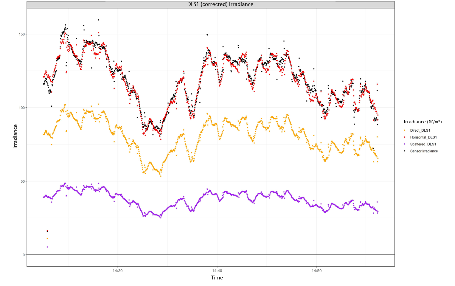
Figure 13.13: Direct, horizontal, sensor, and scattered irradiance across the duration of the flight corrected using the DLS1 method.
Now that we have corrected the data using the DLS1 method (Figure 13.13), we can compare the DLS1 values to the DLS2 values to see if correction is needed. The code below creates a dataframe that has the median scatted/direct ratios and median percent scattered irradiance values for the DLS1 method and from the DLS2 sensor. These values will be used to annotate the comparison plot in Figure 13.14.
Click to show the code
avg_ratio_data <- xmp_corrected %>%
  filter(!is.na(BandName))%>%
  group_by(BandName) %>%
  summarize(median_ScatteredDirectRatio_DLS2 = median(as.numeric(ScatteredIrradiance) /as.numeric(DirectIrradiance), na.rm = TRUE),
            median_ScatteredDirectRatio_DLS1_calc = median(as.numeric(ScatteredIrradiance_new) /as.numeric(DirectIrradiance_new), na.rm = TRUE),
            median_percent_scat_DLS2 = median(100*as.numeric(ScatteredIrradiance)/(as.numeric(ScatteredIrradiance)+as.numeric(DirectIrradiance))),
            median_percent_scat_DLS1 = median(100*as.numeric(ScatteredIrradiance_new)/(as.numeric(ScatteredIrradiance_new)+as.numeric(DirectIrradiance_new))),
            max_Date_time = max(Date_time),
            max_dir = max(DirectIrradiance, na.rm = TRUE)) %>%
  ungroup()%>%
  mutate(
    Scattered_To_Direct_Ratio_DLS2 = as.character(round(median_ScatteredDirectRatio_DLS2,2)),
    Scattered_To_Direct_Ratio_DLS1 = as.character(round(median_ScatteredDirectRatio_DLS1_calc,2)),
    Percent_Scat_DLS2 = as.character(round(median_percent_scat_DLS2,2)),
    Percent_Scat_DLS1 = as.character(round(median_percent_scat_DLS1,2)),
    x = max_Date_time,
    y = max_dir,
  )%>%
  dplyr::select(c(Scattered_To_Direct_Ratio_DLS2,Scattered_To_Direct_Ratio_DLS1,Percent_Scat_DLS2,Percent_Scat_DLS1, x, y, BandName, camera))

unique(xmp_corrected$CenterWavelength) #make sure all wavebands are present

saveRDS(avg_ratio_data,paste0(dir,date,"\\1_Data\\",MS_folder_name ,"\\CSV\\",date,"_avg_ratio_data.rds"))  #SET PATH to save the rds to
Plotting original verse corrected irradiance exif data to compare values from the DLS2 to corrected values using the DLS1 method (Figure 13.14).
Click to show the code
data = avg_ratio_data %>% filter(BandName %in% c("Blue")) # only need to look at one band

(Dir_scat_irr_plot <- xmp_corrected %>%
    filter(BandName %in% c("Blue")) %>%
    mutate(DirectIrradiance = as.numeric(DirectIrradiance),
           ScatteredIrradiance = as.numeric(ScatteredIrradiance),
           Irradiance = as.numeric(Irradiance),
           SpectralIrradiance = as.numeric(SpectralIrradiance),
           HorizontalIrradiance = as.numeric(HorizontalIrradiance),
           # Date_time = ymd_hms(CreateDate),
           Time = format(Date_time, format = "%H:%M:%S"),
           #scaled
           DirectIrradiance_scaled = as.numeric(DirectIrradiance)*0.01,
           ScatteredIrradiance_scaled = as.numeric(ScatteredIrradiance)*0.01,
           SpectralIrradiance_scaled = as.numeric(SpectralIrradiance)*0.01) %>%

    ggplot(aes(Date_time)) +
    geom_line(aes(y = DirectIrradiance, color = "Direct"), linewidth = 1) +
    geom_line(aes(y = DirectIrradiance_new, color = "Direct_DLS1"), linewidth = 1, linetype = "dashed") +

    geom_line(aes(y = ScatteredIrradiance, color = "Scattered"), linewidth = 1) +
    geom_line(aes(y = ScatteredIrradiance_new, color = "Scattered_DLS1"), linewidth = 1,linetype = "dashed") +

    geom_line(aes(y = HorizontalIrradiance, color = "Horizontal"),linewidth = 1) +
    geom_line(aes(y = HorizontalIrradiance_new, color = "Horizontal_DLS1"),linewidth = 1, linetype = "dashed") +

    geom_line(aes(y = Irradiance, color = "Irradiance"), linewidth = 1) +
    geom_line(aes(y = HorizontalIrradiance, color = "Horizontal"),linewidth = 1) +
    geom_line(aes(y = SpectralIrradiance, color = "Spectral"), linewidth = 1.5, linetype = "dotted") +
    labs(x = "Time (UTC)", y = "Irradiance", title = paste0("DLS1 (corrected) vs. DLS2 (metadata) Irradiance, Site: ",site_to_plot,",
                                                      \nDate: ", date_to_plot,", Camera: ", camera_to_plot,
                                                      "\nScattered_To_Direct_Ratio_DLS1:", data$Scattered_To_Direct_Ratio_DLS1,
                                                      "\nScattered_To_Direct_Ratio_DLS2:", data$Scattered_To_Direct_Ratio_DLS2,
                                                      "\nPercent_Scat_DLS1:", data$Percent_Scat_DLS1,
                                                      "\nPercent_Scat_DLS2:", data$Percent_Scat_DLS2
                                                      )) +
    scale_x_datetime(date_breaks = "10 min", date_labels = "%H:%M") +
    scale_color_manual(values = c("Direct" = "blue",
                                  "Direct_DLS1" = "lightblue",
                                  "Scattered" = "black",
                                  "Scattered_DLS1" = "grey",
                                  "Horizontal" = "red",
                                  "Horizontal_DLS1" = "orange",
                                  "Spectral" = "forestgreen",
                                  "Irradiance" ="purple"
    ),
    name = "Irradiance (W/m2/nm)")+
    facet_grid(BandName ~ camera, scales = "free")+
    theme_bw()
)
Figure 13.14: Direct, horizontal, scattered, and spectral irradiance from the DLS2 and DLS1 method from the MicaSense exif data, flown on June 25th, 2024. Average ratio of scattered: direct irradiance componenets for the DLS1 was 0.46 and 0.09 for the DSL2.
Refer to the section Is Correction Needed? to help decide whether your data needs correcting.
Up to this point, we have calculated “corrected” irradiance and sun sensor angles however have not overwritten the exif data within the MicaSense imagery. In this next step, we will overwrite image exif data with the corrected DLS1 values. Before moving on to this step ensure that :
You have decided that your data needs correcting
You have created a backup of your original data, since you will be irreversibly overwriting the exif data of the imagery. Prior to running the code below we copied all images in our MicaSense folder to a folder in the same directory as the MicaSense folder however named named MicaSense_cor. Imagery in the MicaSense_cor folder will be the imagery we will be editing, and the MicaSense folder will contain the unedited imagery
The MicaSense.config has been downloaded from GitHub, the file can be found in the “Scripts” folder under MicaSense
Click to show the code
# Writing over exif data with corrected SSA, horizontal irradiance, direct irradiance, and scattered irradiance

corrected_directory <- paste0(dir,date,"\\1_Data\\",MS_folder_name,"_cor\\") #i.e. this folder is called MicaSense_cor and is a copied version of the MicaSense folder, we will be correcting the exif data of images in the MicaSense_cor folder and leaving the MicaSense folder untouched with the original exif data
original_directory <- paste0(dir,date,"\\1_Data\\",MS_folder_name,"\\") # path the folder of micasense images

xmp_corrected = readRDS(paste0(dir, date, "\\", MS_folder_name,"\\CSV\\",date,"_xmp_corrected.rds")) %>% #path to corrected xmp data .rds file
  mutate(SourceFile = str_replace(SourceFile,original_directory, corrected_directory), # Changing source file name from the original directory to the corrected_directory. This will result in imagery in the corrected direcotry only to be edited
         TargetFile = SourceFile) #the TargetFiles are the path names to the files to be edited

# As vectors
(img_list = xmp_corrected$FileName)
(targets = xmp_corrected$TargetFile)
(SSA = xmp_corrected$SunSensorAngle_DLS1_rad)

(horirrorig = xmp_corrected$HorizontalIrradiance)
(horirr = xmp_corrected$HorizontalIrradiance_new)
(dirirr = xmp_corrected$DirectIrradiance_new)
(scairr = xmp_corrected$ScatteredIrradiance_new)

targets[1] #checking its the right imgs

for (i in seq_along(targets)) {
  # given a micasense config file, overwrite tags with computed values
  # using exiftool_call from the exifr package
  call = paste0("-config G:/GitHub/GenomeBC_BPG/MicaSense/MicaSense.config", # SET PATH to the config file, this file is on the PARSER GitHub in the same folder as this R script
                " -overwrite_original_in_place",
                " -SunSensorAngle=", SSA[i],
                " -HorizontalIrradiance=", horirr[i],
                " -HorizontalIrradianceDLS2=", horirrorig[i],
                " -DirectIrradiance=", dirirr[i],
                " -ScatteredIrradiance=", scairr[i], " ",
                targets[i])

  exiftool_call(call, quiet = TRUE)
  print(paste0(i, "/", length(targets), " updated img:",img_list[i] ))
}
Lastly, check the exif data of the first and last image to ensure that the data has been properly overwritten.