Chapter 8 Georeferencing Plot Trees

At this stage in the workflow we have processed high quality imagery into orthomosaics ready for analysis. The next step is to georeference the row and column census data and the high quality P1 template to geolocate the trees, which will be used later on to create individual tree polygons. Figure 8.1 is an image of the spreadsheet map from the Big Tree creek site which is typical of many BC genetics trials. Figure 8.2 is the P1 orthomosaic template flight we georeference the census data to.

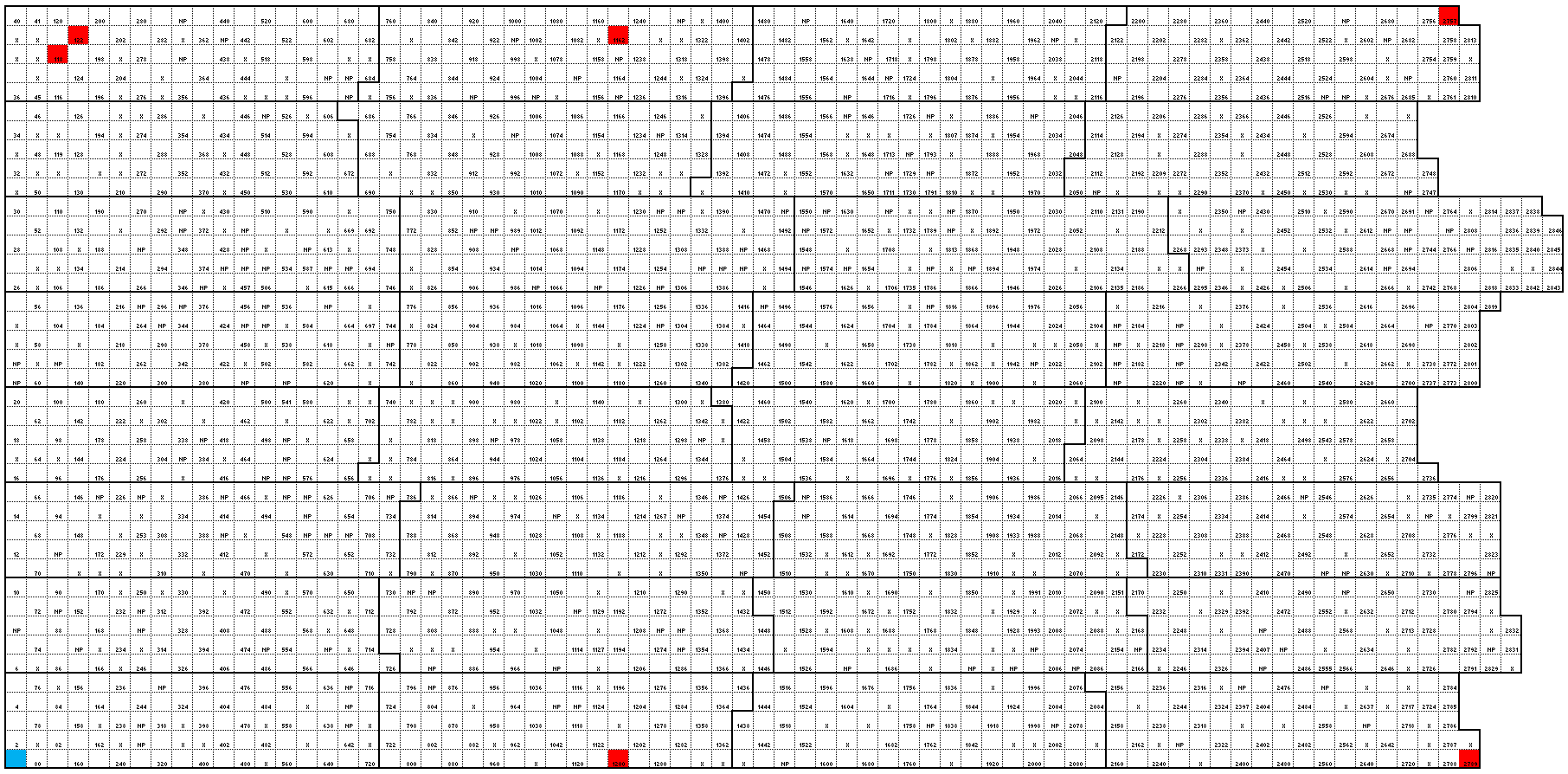
Figure 8.1: The spreadsheet map of the layout of the site, each tree is located on a grid with a unique row and column value assigned to it.

Figure 8.2: P1 orthomosaic of the site with GCPs and georeferenced trees marked with red dots

We have recently developed a “Grid Georeferencer” plugin in QGIS that does the initial rough georeferencing of the census data and is available for download here. We also have a version that works in R. Both are detailed below.

8.1 Workflow in QGIS

The census data is examined, and a unique identifier column is found or created.
1. This column is “treeID” and will be used through the rest of the data processing pipeline.
2. The census data must also contain “row” and “col” (row and column identifiers).
The information from the reconnaissance workflow is used to locate reference trees.
1. The distance, Azimuth and treeID from each GCP to the nearest plot tree was recorded as a reference tree.
2. In a GIS (in this case QGIS) a shapefile is made with the reference trees. They are visualized as red dots in Figure 8.2. The shapefile is saved in the “working” reference system NAD83 UTM’s.
The Grid Georeferencer plugin is run in QGIS as seen in Figure 8.3. This plugin:
1. builds the grid based on the row and col fields at the spacing input.
2. rotates the grid based on the input reference trees and saves a copy of this rotated version as “_rotated” in the export folder.
3. applies an affine transformation to better fit the grid to the reference trees. It saves this as “_transformed” and loads it into QGIS.
- To run the plugin (see Figure 8.3):
  - enter the Input csv and choose the extra fields to import
  - enter the grid spacing
  - enter the export location

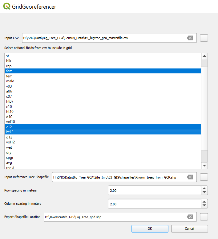
Figure 8.3: Visual of the Grid Georeferenced plugin in QGIS.

8.2 Alternate Workflow in R

The Grid Georeferencer plugin described above was created by our team to make grid georeferencing easier for uptake. Here we describe our original method, based in R, for those who choose to keep their workflow in R

Follow steps 1-2 from the Workflow in QGIS

Identify the tree that is in the first row and first column and first row and last column:
- Here the tree in the first row and first column is the bottom left tree shown as a blue dot in Figures 8.1 & 8.2). Export this tree as a shapefile which will be read into the below R script as “first-first”.
  - ** Note ideally we would have a GCP at the bottom left corner of the site however, this was the densest section at this particular site, so the columns and rows were carefully counted in either direction from the nearest reference tree instead.
- The tree in the first row and last column is the bottom right tree in Figures 8.1 & 8.2 and coincidentally a reference tree next to GCP_2 (Figure 8.2). Export this tree as a shapefile which will be read into the R script as “first-last” below.
Run the R script that will create a grid with the correct orientation and spacing to match your plot trees. The R script can be found here or in the code chunk below. ** Note this script requires North up rows and East up columns to work as scripted. Modifications will need to be made to sites with different orientations. This code will install the required libraries, set up the file structure as we use it and follow these steps:
1. Read in the shapefiles for the first-first and first-last trees.
2. Load the CSV file, filter for the required columns. At Big Tree we want the row, col, treeID and the most recent assessments, which here are a 2012 remeasurement (ht12) and assessment (c12).
3. Generate Initial Grid: Create a grid of tree locations using the row and column numbers, starting from the initial point (first-first). Adjust the coordinates to account for column and row spacing.
4. Convert to Spatial Object: Convert the grid data to an sf (simple features) object in R.
5. Identify Reference Point: Extract the coordinates of the tree in the first column and the last row (first_last_sf) from the grid.
6. Calculate Rotation Angle: Define a function to rotate coordinates. Calculate the angle of rotation needed to align the grid with the actual positions of the initial points.
7. Rotate Grid: Apply the rotation to all points in the grid.
8. Merge and Save Results: Merge the rotated coordinates with the original grid data. Set the CRS and save the resulting grid as a shapefile.
9. Plot Final Grid: Plot the final rotated grid to visualize the tree locations.

Click to show the code

library(tidyverse)
library(sf)
library(sp)

dir = "Q:\\SNC\\Data\\Big_Tree_GCA\\"
name <- "Big_Tree"
csv_path = paste0(dir, "Census_Data\\#4_bigtree_gca_masterfile.csv")
trees <- paste0("Site_Info\\03_GIS\\shapefiles")
#shapfiles for the below trees were done in a GIS off high res imagery
first_first = st_read(paste0(dir, trees, "\\first_first.shp")) %>% 
  st_geometry()
first_last = st_read(paste0(dir, trees, "\\first_last.shp")) %>% 
  st_geometry()

# column spacing in m 
c_space = 2
# row spacing in m 
r_space = 2
# read in the CSV
(csv_B = read.csv(csv_path) %>% 
  dplyr::select(treeID, row, col, ht12, c12))
# produce a grid using row and column numbers, to be rotated
grid = csv_B %>% 
  mutate(
    x_coord = st_coordinates(first_first)[1] + (col * c_space) - c_space,
    y_coord = st_coordinates(first_first)[2] + (row * r_space) - c_space)
# to sf object
grid_sf = st_as_sf(grid, coords = c("x_coord", "y_coord"), crs = 26910)
# get the coordinates of the first-last
first_last_sf = grid_sf %>% 
  filter(row == 1) %>%
  filter(col == max(.$col)) %>% 
  st_geometry()
# define a FUNCTION which rotates coords for a given angle
rot = function(a) matrix(c(cos(a), sin(a), -sin(a), cos(a)), 2, 2)
# get the angle of rotation between the true (first, last) and
# the current position of (first, last)
a = st_coordinates(first_last - first_first)
b = st_coordinates(first_last_sf - first_first)
theta = acos( sum(a*b) / ( sqrt(sum(a * a)) * sqrt(sum(b * b)) ) )
# rotate all points 
grid_rot = (st_geometry(grid_sf) - first_first) * rot((theta)) + first_first
# in order to merge the new coordinates and the census info, copy the sf object created from the master csv
grid_rot_sf = grid_sf
# then replace its geometry with the rotated coords
st_geometry(grid_rot_sf) = grid_rot
# and set its CRS to the correct one
st_crs(grid_rot_sf) = 26910
#save rotated grid
st_write(obj = grid_rot_sf,
         dsn = paste0(dir, trees, "\\", name, "_grid_manual_bpg.shp"),
         append = FALSE,
         crs = 26910)
#plot(grid_rot_sf) #uncomment to plot the rotated grid

8.3 Final Steps in QGIS

The grid is loaded into the GIS and examined. The first-first corner with row 1 column 1 looks great, but the top right corner is at least 2 meters off as you can see below. This is one of the better ones we have georeferenced. The site is on even ground and was quite square. Some of the sites were 6 meters off from one corner to the other.

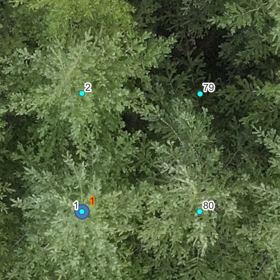
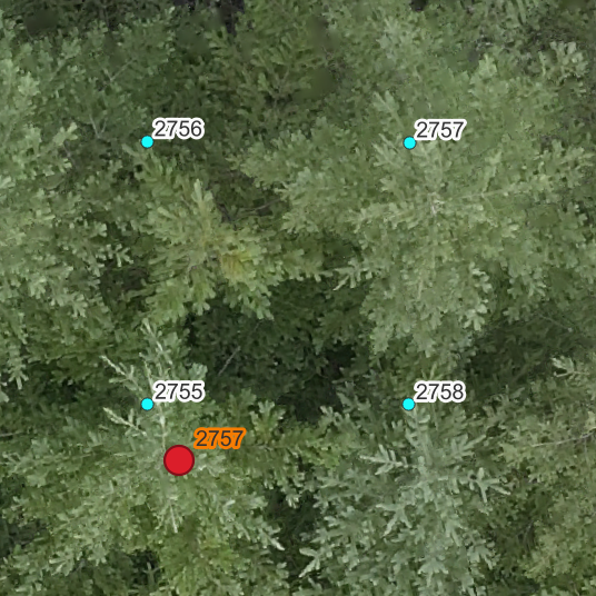
Figure 8.4: Left: treeID 1, reference for the bottom left corner of the plot. Right: treeID 2757, reference for the top right of the plot

We now use the reference trees and QGIS’ Georeferencer plugin if needed to tighten up the fit of the grid to the Orthomosaic. Open the Georeferencer and select the Transformation Settings icon as seen to the left. The polynomial 2 transformation works well, but another transformation can be tried if it doesn’t fit. Once sufficient, add the vector layer that we exported from R and zoom in on the first point that matches a reference tree as below. Then add a point and select the From Map Canvas button.

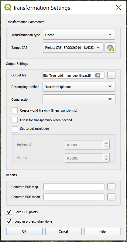
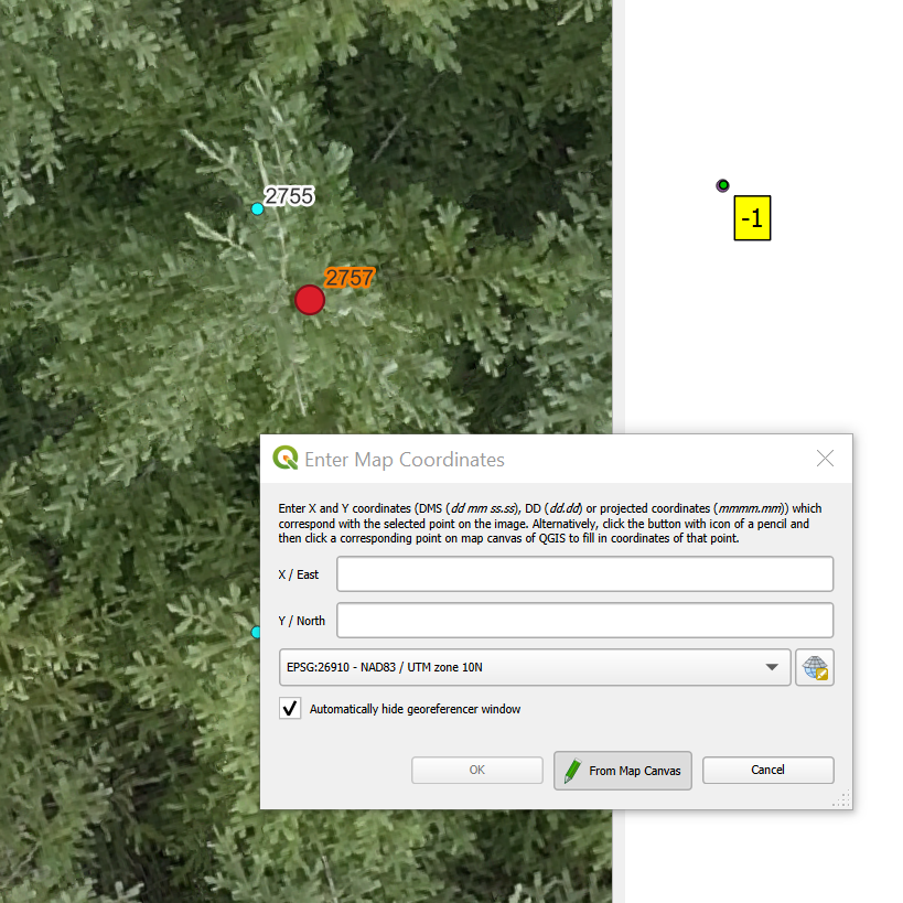
Figure 8.5: Left: Transformation settings. Right: zoom in on vector layer and place a point on the Map Canvas

Work through the reference trees. With 6 reference trees spread evenly through the site the fit was quite good as seen here.

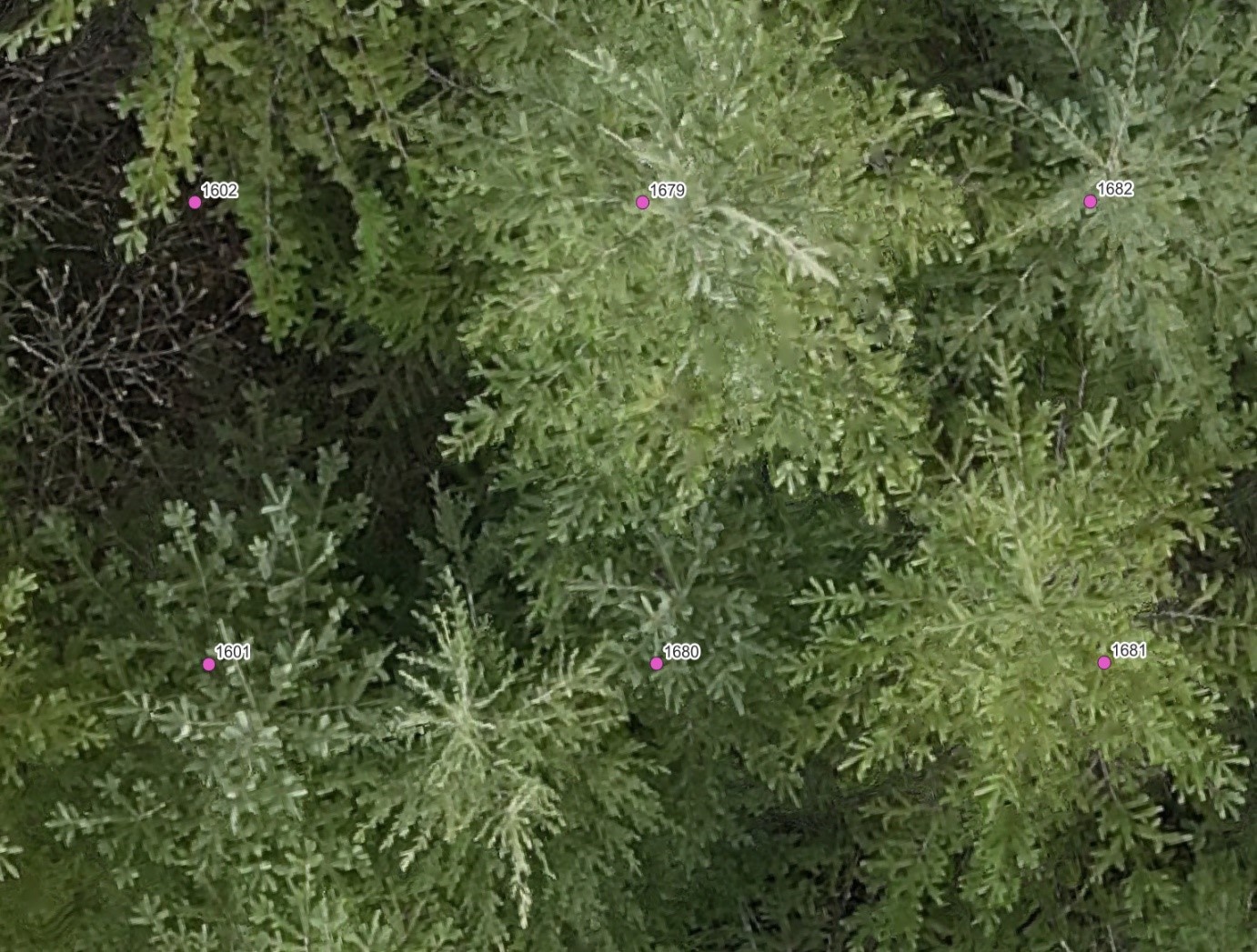
Figure 8.6: Zoomed in visual of the georeferenced tree grid for 6 trees overlain on the P1 orthomosaic.

From here we will manually move each tree position to its visible top. This is a time-consuming task, as care must be taken. In the above imagery the tree between 1601 and 1680 is ingress (a Western hemlock, not planted as part of the trial), the P1 imagery helps to make the distinction visible. On sites that have been recently maintained as pictured below, and if you already have a CHM, a time saving method is to buffer 30-40cm circles around your tree points, then snap the tree point to the local maximum. This can be done in R or a GIS.

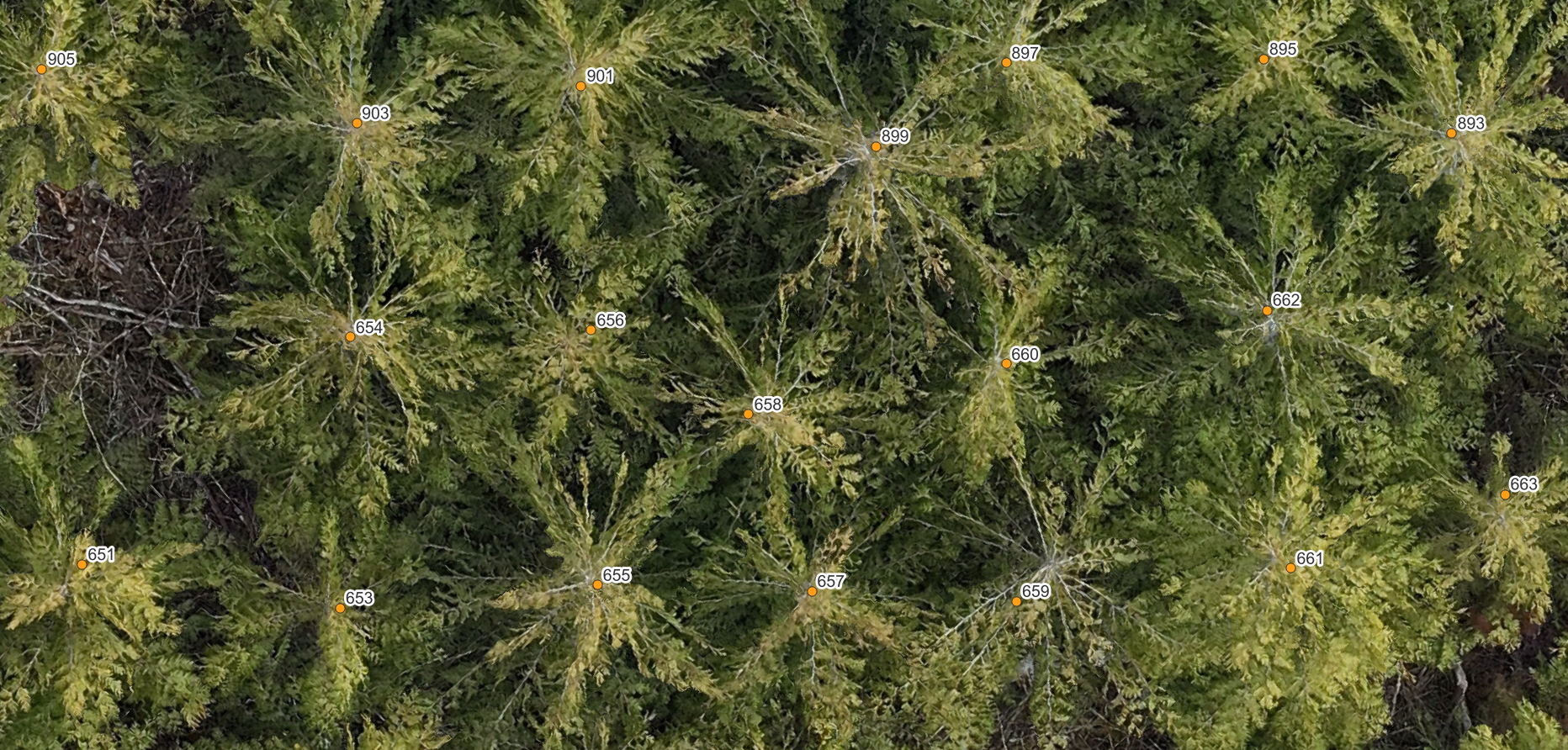
Georeferenced grid overlain on P1 orthomosaic for a site that was well maintained. The georeferenced grid has been snapped to the highest point on the CHM within a given radius to pull the grid to the treetops.

Figure 8.7: Georeferenced grid overlain on P1 orthomosaic for a site that was well maintained. The georeferenced grid has been snapped to the highest point on the CHM within a given radius to pull the grid to the treetops.